Exploring Digital Spectral Band Concepts through Satellite Imagery

Introduction:

In this lab, we were tasked with using the ESRI Landsat Application in order to analyze and study satellite imagery using various spectral bands. Following the tutorial that ESRI has created, we viewed numerous locations and scenarios changing the bands to identify key aspects and information of each area. The different bands used were very useful in collecting data that could be used in various different industries. These specifics will be discussed throughout this post.

Objectives: 

#1: Discover, identify, and apply the capabilities and options of working with a temporal raster data set

#2: Recognize, relate, and compare the similarities and differences between UAS data and Satellite data

#3: Demonstrate proficiency and knowledge on how to effectively utilize spectral bands to given applications and identification of objects.

Color Infrared:

Looking at the Sundarbans on the border of India and Bangladesh, we enabled the Color Infrared band combination that completely changed the coloring of the default map. The land areas became a bright red and the areas of water became a light blue. (Figure.1) This color band is immensely useful when determining vegetation health in areas. Something to note is the various shades of red scattered throughout the area. The brighter the red, the healthier the vegetation is and, conversely, the darker the red, the less healthy the vegetation is. In order to get a better understanding of the color infrared combination, I zoomed into an area near Purdue and captured a screen shot with the same band on. (Figure.2) The areas off to the west of Purdue were a very dark red and there are even some areas that have no red at all. This color band can very crucial for the agriculture industries when trying to determine the health of their crops which can reduce the large amount of time that is allocated to individuals walking around inspecting plants by hand.

(Figure.2 Purdue w/ Color Infrared)

(Figure.1 Sundarbans w/ Color Infrared)

Index:

Next we viewed the Taklamakan Desert using the Moisture Index. As opposed to the Color Infrared Band's combination of three spectral bands, the Moisture Index is "a calculation that adds and divides the values of various bands to find moisture-rich areas." This index highlights the areas that have noticeable amounts of moisture in blue. (Figure.3) It is very similar to the Color Infrared in the sense of the information it can display. However, something to note, is that large areas of blue on the map are not necessarily bodies of water. These can be areas of vegetation that have large amounts of moisture. While it can display healthy vegetation like the color infrared, this index is aimed towards identifying areas that are moisture-rich. Along with the Moisture Index, we also viewed the Agriculture band combination. This combination highlights areas of agriculture in bright green. However, the key component of this map is that agriculture and bodies of water can be distinguished because it does not just highlight areas that have moisture but instead areas of vegetation (Figure.4)

(Figure.3 Moisture Index)

(Figure.4 Moisture Index)

Temporal Resolution:

The time tool in the Landsat application is incredibly useful for identifying the changes of a location over a period of time. This tool allows the user to look at a specific location and the periods over time that it was recorded. Below are images of Las Vegas, Nevada from the earliest point in time (Figure.5) it was recorded and the most recent point in time. (Figure.6) You can definitely see the development of the city and the changes in landscape, especially in the bottom right corner of the images. 

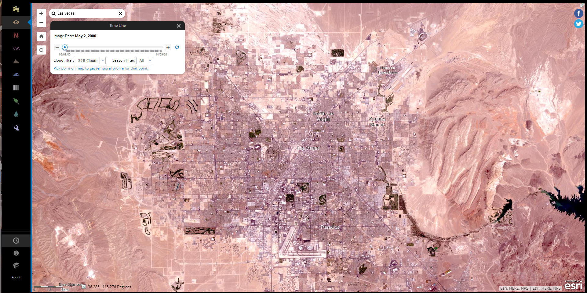(Figure.5 Las Vegas, NV Earliest Time)

(Figure.6 Las Vegas, NV Most Recent Time)

The next 2 images are from Phoenix, Arizona with the same temporal change. Again, with Phoenix, you can see the development of the city and how the landscape has changed over time. (Figure. 7 & 8)

(Figure.7 Phoenix, AZ Earliest Time)

(Figure.8 Phoenix, AZ Most Recent Time)

Creating My Own Spectral View:

In this section of the assignment we were tasked with combining various bands to create our own spectral view. I created 5 different band combinations and each are listed below with their respective images and locations.

East Coast of Japan:

Much of the land in this band was red with some dark gray areas. I can assume that the areas in dark red are vegetation because of the NIR band

NIR(5) + Red(4) + Green(3)

(Figure.9 East Coast of Japan)

Purdue University:

The map looks somewhat normal to what we would normally see. The vegetation has different apparent colors than that of the residential areas. Some of the less dense areas of population are kind of hard to differentiate.

SWIR(7) + SWIR1(5) + Coastal(1)

(Figure.10 Purdue University)

Dallas, Texas:

The map has a purple/blue tint to it. The areas inside the city are a dark yellow and the areas that do not have as many residents are deep purple.

Red(4) + Coastal(1) + Cirrus(8)

(Figure.11 Dallas, Texas)

Terre Haute, Indiana:

The map is extremely blurry and very fuzzy. the areas of agriculture are a tan color while what seems like forests are a dark blue. The areas of population are blurry but I can still make them out.

SWIR2(7) + Green(3) + Cirrus(8)

(Figure.12 Terre Haute, Indiana)

Ansbach, Germany:

The map has mainly different shades of blue. Populated areas have a yellow hint but otherwise most of the areas of agriculture are different shades of blue.

Coastal(1) + Blue(2) + SWIR1(6)

(Figure.13 Ansbach, Germany)

Discussion: 

In this lab we used the Landsat application by Esri to analyze various forms of spectral bands and tools. Through this I gained a better understanding on how to use one of the many tools that the UAS industry has at its disposal. Viewing data in different bands can show data and information that would not normally be present. For example, being able to view the vegetation health of an area by simply enabling a band. These types of tools are invaluable to the GIS industry.